


The Stern-Gerlach Experiment : Part 1
Atomic spin, magnetic moments and how to measure them.

We sketch the Stern-Gerlach experiment which proved the quantization of spin angular momentum. We define in detail what a magnetic moment is, and how they are related to atomic spin. Finally we discuss the physics of how the Stern-Gerlach measurements are made.
Last time we mentioned that angular momentum was quantized in units of Planck's constant, h. That's the same h that was used to quantize the energy levels of the hydrogen atom. As we've been saying, h sets the resolution for information density in space and time.
Today we'll discuss how we know that spin angular momentum is quantized. That is, we'll review the first experiment designed specifically to test this hypothesis. Understanding how the experiment worked will set the scene for learning the technical details that will let us use the mathematics to describe quantum systems and quantum bits - or qubits - of quantum logic.
The Stern-Gerlach Experimental Design
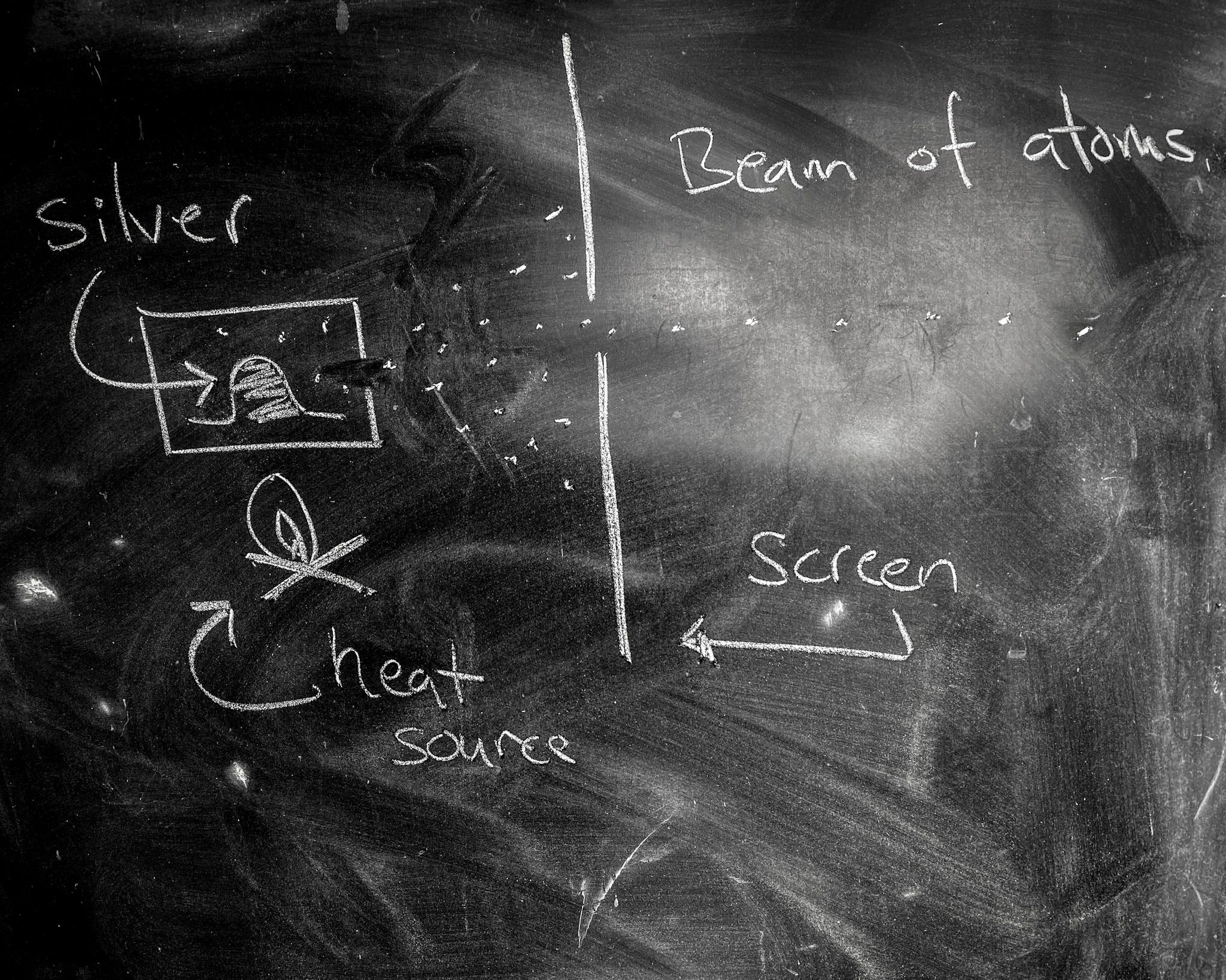
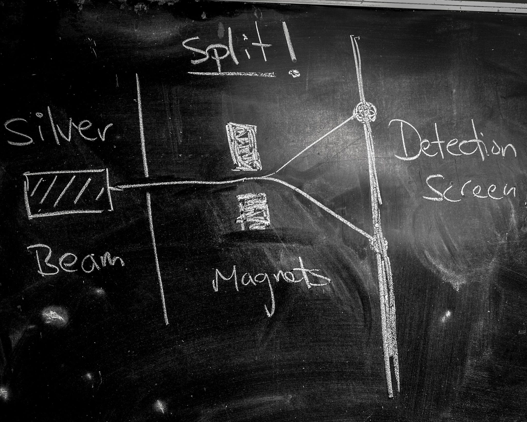
The quantization of spin angular momentum was first demonstrated by explicit experiment by Stern and Gerlach in the 1920's1. The basic idea was to take a beam of silver atoms and fire them at a large, sharply pointed magnet. The large magnet would push on the atoms in proportion to their spin-associated dipole magnetic moment. If spin were truly quantized, so too would be the magnetic moments and the beam would be split. If it were not, the beam would be smeared.
Of course, the beam was split.
Silver atoms were chosen because Quantum Mechanics predicts that their spin angular momentum is quantized to either ±h/4π. The beam of silver atoms was achieved by heating a lump of silver metal inside a box with a pinhole opening. Atoms of silver would sublimate from the lump and occasionally leave through the pinhole. A second, filtering pin hole screen could then be used to focus these errant atoms into a beam.
What is a Magnetic Moment, Exactly?
So far, we've thought of the magnetic field of a particle - like a silver atom or an electron - as a dipole field that looks qualitatively like the Earth's magnetic field, only smaller. The precise mathematical description of a dipole field can get rather complicated.
One way to think of a magnetic dipole moment is as a vector parameter for a dipole magnetic field2. From this perspective, with m as a constant vector, the overall magnetic field at a point as a function of the position vector r is:

Evidently the parameter m the magnetic moment - is much easier to work with.
Last time we mentioned that these little dipole moments tend to align against the presence of an a large, external magnetic field, B. The cause of this alignment is a torque which is easy to express in terms of m:

This torque gives us another way to think of m. We can turn this classical idea around and use (1) to define the constant dipole vector m as how strongly the particle torques in the presence of a constant magnetic field. This can then be considered an experimental observable that describes the physical magnetic field generated by the particle.
Magnetic Fields and Force
Last time we saw that the tiny magnetic moments of individual particles are affected by an external magnetic field. Specifically, the potential energy U of such a particle with a tiny magnetic momentum m is given by

Unlike the defining relation (1), (2) is true regardless of whether B is a constant, large, magnetic field. In particular, the experiment of Stern and Gerlach utilizes an external magnetic field with a sharp variation in position.
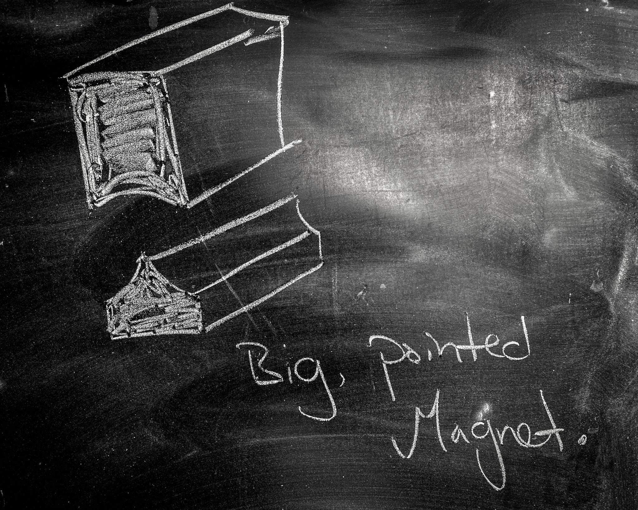
This can be arranged, as we mentioned, by taking a really strong magnet with a very pointed shape.
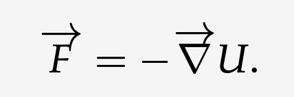
When B depends on position (but m is still constant), we can take the gradient to find a force:
The force will depend only on the gradient of B:

This is a terrifying expression! But of course it is, it's too generic. It holds for any generic big magnetic field B.
Let's simplify things a bit by designing our magnet so that

In other words, the magnet only varies in one direction, and that's the x-direction. This simplifies our force by knocking out the second term,

As a result, (3) tells us that there is a force proportional to the directional derivative of B along the direction m. In other words if m is parallel to the spike in the magnet, the force is biggest. If it's perpendicular to it, there is no force.
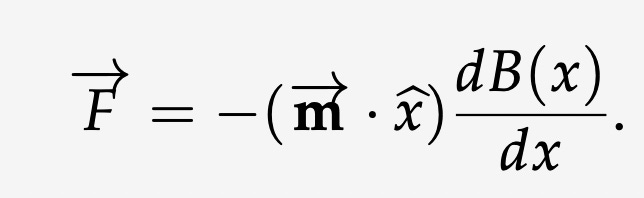
If you like, we can write this purely in the x-direction:
A Quantized Force
And so we see the clever design behind the Stern-Gerlach experiment. If the magnetic moments of individual particles like atoms really is quantized in units of h, then for a given magnetic field B, the force should be quantized, too!
For the simplest case, like the silver atom, where
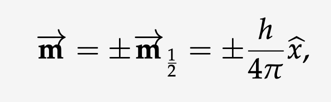
there are only two options for the force on a particle:

“Very nice!,” you might say, “Except for one thing. What happens when m runs perpendicular to x?”
The short answer is simple: the force is still given by (4).
“Surely, that's wrong!” You might say again. “Doesn't (3) show that the force should be zero if, say, m is orientated along the y-direction?”
And now we see what we mean when we say that h puts a finite resolution on information - in this case the spin angular momentum of individual particles. The universe can only answer this question in units of h/4π. In any given direction, x, y or z, the spin angular momentum of a silver atom is either ±h/4π. It's never zero. The force still ±|F|. Which direction, ±F, is chosen by nature, at random.
What's fascinating about particles like silver atoms or electrons, is that there are only two possibilities. In particular, 0 is not among those possibilities. What is true, however, is the the average value of the spin angular momentum - averaged over all the atoms in present in the beam - can be zero.
To better understand this short answer, we probably should discuss the long answer. And the long answer is the subject of our next discussion.
Nobel Laureate Dudley Herschbach has a great write up about the history of the experiment. [doi/10.1063/1.1650229]
See, for instance, page 186 Dave Jackson’s text “Classical Electrodynamics” or D.J. Griffith’s “Introduction to Electrodynamics.”