


Putting a finer point on it.
Path Integrals and the auxiliary importance of waves.

Science applies mathematics to quantify empirical findings. If done well, these findings also quantify their uncertainty. What makes Physics so powerful - and so philosophically confounding1 - is that newer models nest into older ones as we reduce this uncertainty.
Put differently, older models in Physics don’t get rejected by new information, they get refined.
What’s interesting about Quantum Theory is that nature introduces its own, intrinsic error. Reality is stochastic. There really is a fundamental limit to our knowledge of the physical world.
Our previous discussion involved the idea of particles in different regimes, from Classical Mechanics to Quantum Mechanics to Quantum Field Theory:

In that piece I argued dismissing the idea of a “particle” was a semantic issue, not a Scientific one. Today I’d like to refine this claim by exploring exactly how the idea of a classical particle embeds into Quantum Mechanics and subsequently Quantum Field Theory.
The main tool for this will be the Path Integral formulation of Quantum Mechanics. In my view, the wave-particle duality obfuscates the Physics of Quantum Theory. To better understand particles and matter we will use Path Integrals. Path Integrals involve a fixed recipe that works for particles, fields, strings or even fields of strings. It works for any consistent physical system you can write down2.
Let us begin.
Particles, Redux
A classical particle is modeled by a point - that which has no extent in any dimension. It often comes equipped with extra data, like a mass or an electric charge. Pragmatically, we often think of this as an idealization of something that might have some extent, like a pebble when viewed from far away.
Fundamental particles of course should not have any such structure, and should be point-like at any resolution of observation. The wave-particle duality is crude way of expressing the fact that Quantum Mechanics introduces its own, fundamental error in any possible observation of that particle. It is this inherent error that adds nuance to the classical ideal of a particle.
The Principle of Least Action
The Action gives a traditional way of defining a model for a physical system. The action for a classical particle of mass m can be written as a simple integral3
Here s is a parameter along the path of a particle as it moves through space and time. The path the particle takes is represented by γ. The longer the path, the greater the action. In other words, the action is a line integral in four-dimensional spacetime
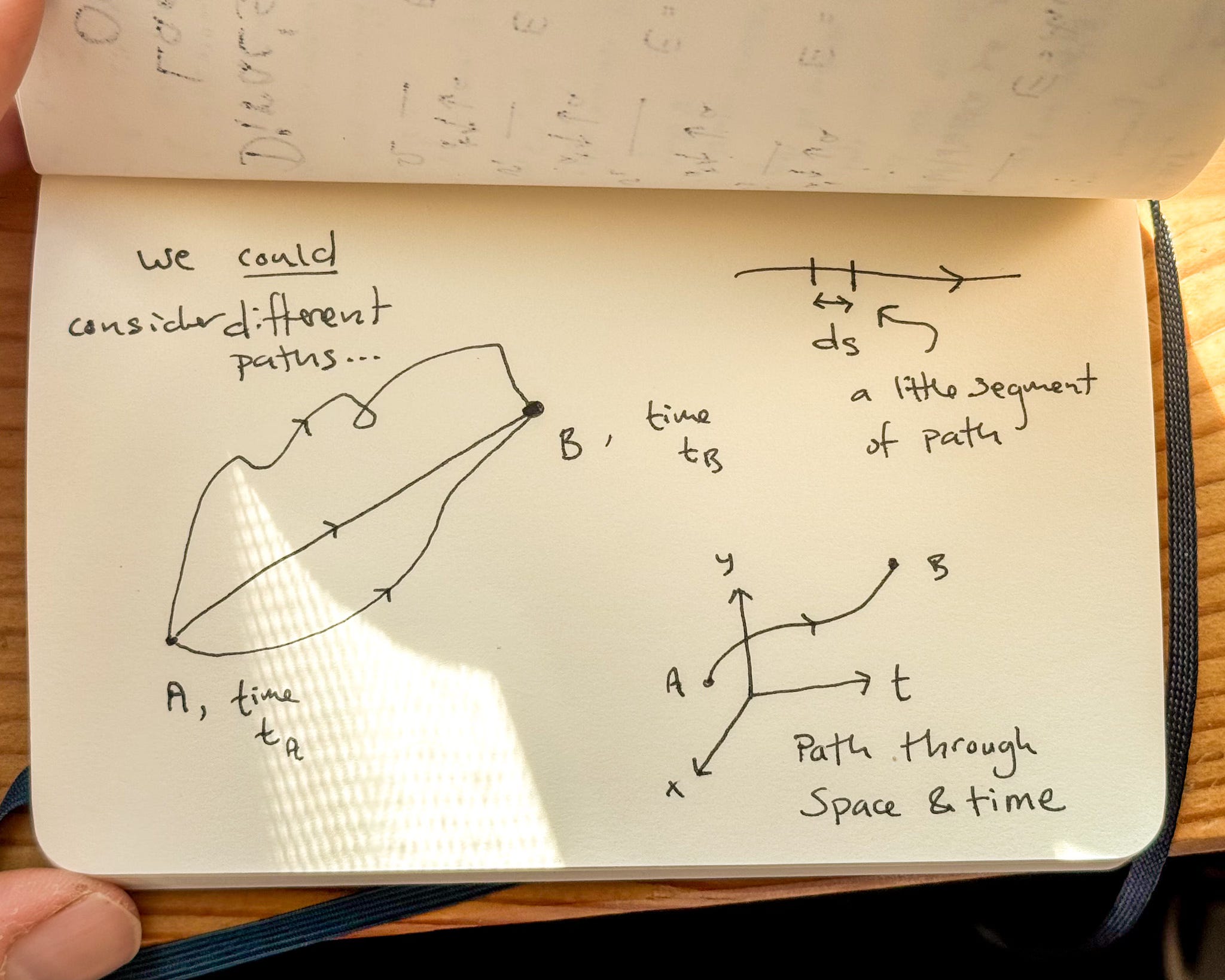
The Principle of Least Action states that the path a particle takes is the shortest one - that is, the one for which S(γ) takes the smallest value. The practice of Physics then gives a generic algorithm for computing the path γ which minimizes S(γ).
Let us call the path that minimizes4 the S(γ) is called the classical path of the particle.
Here are some additional details independent of the main line of argument:
We are glossing over a lot of technical details. Finding the shortest path through space is one thing, but what determines the velocity of the particle? Additionally, a shortest path implies that we know where the particle is going ahead of time. What if the terrain is hilly or has a cliff or a pond to contend with? How can we be sure that the path even exists?
The answer to these questions requires including enough detail to completely define the problem. In this case, we need to ask what is the shortest path between some two fixed points in space and time?
Practically, this involves a differential equation for which these two fixed points serve as boundary conditions. Other methods in Physics - such as Newton’s Laws - can give rise to the same differential equations, and will also require the same data to fully specify the problem5.
It is entirely possible that a given differential equation - with specified boundary conditions - has no solution, as you might expect for the case of a pond or a cliff present in the terrain. If you insist on solving the problem that includes traversing such obstacles, you’ll have to modify the behavior of the particle to include things like forces. This makes the definition of the Action slight more complex. Let’s ignore those details for now so we can move on to Quantum Mechanics.
The Action Principle and Quantum Mechanics
Quantum Mechanics introduces fundamental error into our observations. The particle-wave duality is one interpretation of that error. That particular interpretation was the point of view Strassler took when he defined the term “wavicle”.
Another interpretation of Quantum Mechanics - attributed to Richard Feynman - is easy enough to state: a particle traverses all possible paths between two points in space and time simultaneously.
What is interesting about this interpretation is that the particle retains classical identity, a priori. Its wave-like nature can be seen as an emergent parametrization of the error associated with managing an infinite number of paths.
I’ll sketch that relationship for you now.
The Path Integral
Nature is stochastic. Computing the probability of a particle moving from one point in space and time to another involves computing a weighted sum over all possible paths that particle could take.
To be more precise, the action S(γ) for each path γ gives a different numerical value. We weight the importance of each path γ by a numerical factor W based on S(γ).
W(γ) is a complex phase - a complex number of unit magnitude effectively parametrized by an angle. As we vary the path γ, the phase angle changes. Famously, Euler demonstrated6 that complex phases can be expressed as trigonometric functions,
In some sense, this relation where the wave-like nature of particles comes from.
To be even more precise, we know that as θ changes, the trigonometric functions oscillate between -1 and 1. Hence if S(γ) changes rapidly, to too does θ, and the relevant numbers rapidly oscillate between -1 and 1. Summing over all possible paths weighted by W(γ) means that when the action changes very quickly, we are essentially averaging to zero. This fact is violently exacerbated by the factor of ℏ in the denominator, which means we are dividing by a very, very small number7:
Hence, the only contribution to the sum of paths that does not quickly average to zero are those where the weight W(γ) changes very slowly, which we now investigate.
The main contributions to the Path Integral
We know from differential calculus that the rate of change of a function is given by its derivative. So schematically8 we can compute,
We now know three important things.
The rate at which the path weight W(γ) changes is directly proportional to the rate at which S(γ) does.
Derivative calculus tells us that a local minimum for a function occurs only if its derivative vanishes.
Finally, we know that the classical path minimizes the action S(γ).
Therefore W(γ) changes very little only for paths that are very close to the classical path. What measures what we mean by close? The physical parameter ℏ.
At the smallest scales of matter, we don’t just see particles on their classical paths. Rather, we see the collective action of particles moving through many paths near the classical one. Just as with waves, the phase angle θ - representable by S(γ) - can cause probabilistic interference between the different paths the particle could take.
The wave-particle duality just happens to be an alternative way to interpret this fact.
The Action Principle and Quantum Field Theory
What’s fun about Feynman’s approach to Quantum Mechanics is that it generalizes immediately to any physical system that can be described by an Action. In particular, we can do Quantum Field Theory in exactly the same way.
Of course, the snag here is that we need to write the action for a field instead of a particle. Instead of summing over paths of particles to do physics, we need to sum over continuously connected configurations of a field between two points in time. Put differently, we are summing over histories of the field.
Particles and Waves are still just words
And now we arrive at the source of Strassler’s semantic ire. The classical equation of motion for a free scalar field is just the wave equation. Hence, classical histories of the scalar field which we sum over to compute the path integral are histories of waves propagating through the classical field itself.
But where do the fields themselves come from? And how are they related to particles as we’ve known them?
Just as we’ve seen how summing over all paths of a single particle could be interpreted as a wave, it might be more conceptually pleasing if we could construct some sort of action that captures the set of all possible paths of all possible collections of particles simultaneously, which might then have some interpretation as a field.
Except, this is exactly what a free9 field represents.
The wave-like nature of particles runs deeper than the study of Schrödinger’s wave mechanics. It’s a relationship first explored back in the 17th century, known today as Huygen’s Principle. It grew into Fourier’s representations of continuous functions in the early 19th century.
Particles - when viewed from a spacetime perspective - aren’t points. They’re continuous paths, and what are paths if not functions from time into space.
Linear analysis on the space of functions - and free particles or fields certainly quality as linear - are representable by harmonic functions, of which waves are the archetype.
The Gory Details are important here!
When we do an actual computation that attempts to model a collision of particles in Quantum Field Theory, we see the “wavicle” model for what it is: a semantic expression for abstract algebra, borne from a particular representation of that mathematics.
Let me explain this by sketching the gory deals of a particular calculation.
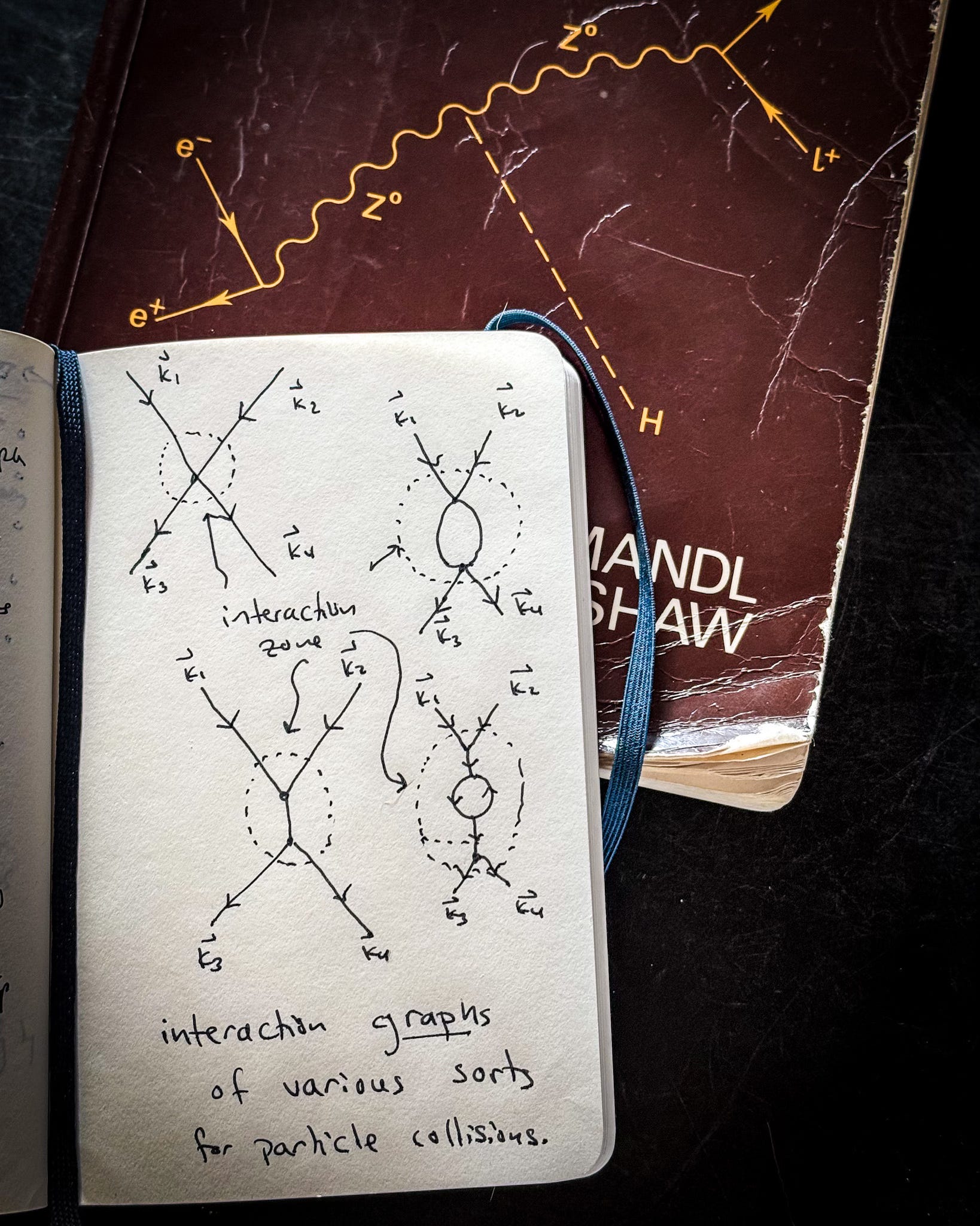
When modeling the output of particle collisions we typically use the so-called interaction picture of Quantum Field Theory. This is essentially the same thing as the time-dependent perturbation theory of Quantum Mechanics. The basic idea is this:
We assume some particles of fixed energy and momentum arrive from very far away. We model them as noninteracting particles for most of the journey. At some point in their path towards each other, we “turn on” the interaction and proceed see what happens. After the particles interact, some other particles will come out and eventually escape to the detector. We similarly “turn off” the interaction when they are sufficiently far away from the interaction zone. This effectively carves out a clean, idealized sphere in space in which we can make the computations as simple as possible.
Yes this is a computational convenience, but it works because of the algebraic structure of Quantum Field Theory10.
In this language, the incoming and outgoing particles are typically represented as fixed-momentum excitations of some quantum field. Mathematically these are represented by plane waves - or wavicles - at Strassler has suggested.
Put explicitly, plane waves from outside the interaction zone are just a method to produce integrals of the form
This expression is an auxiliary factor to the main computation. It is a computational artifact used to enforce the conservation of momentum and energy. The integral over all points in space11 used to enforce the conservation of momentum corresponds to the sum over all possible places where the particles could have collided.
The main part of the calculation actually predicts how the two incoming particles exchange energy or momentum12.
The End Result of the Full Calculation is Particles
Did you catch that? We’re summing over all places where the interaction could have occurred. That is just another manifestation Feynman’s sum over histories approach to Quantum Mechanics.
Fundamentally, these kinds of computations in Quantum Field Theory have the following components:
Particles enter. They trace all possible paths from far away to the interacting region. We sum over all possible action weighted paths for this to happen. Expressing them as plane waves is a mathematical convenience.
Particles interact. We sum over all points in the interacting region where those particles could have interacted. This is basically the sum over all possible histories - or ways the particles could have interacted.
Particles depart. They trace all passible paths from the interaction region to the detectors. Expressing them as plane waves is a mathematical convenience.
Enforce conservation of energy and momentum. The mathematical convenience of plane waves makes this easy to accomplish.
In Quantum Field Theory particle interactions always occur at individual points in space and time. This is how the Action function for fields S(γ) is constructed. This is why the method of Feynman Diagrams involves graphs. The vertices themselves give away the game. Particles are point-like because they interact at points13
The more precise the model used, the more nuance those vertices will have. Exploring the modern theory of Renormalization is a great place to start if you’re interested in these finer points.
TL;DR : Don’t take your ideas too seriously
Particles exist. Fundamental particles exist. The particle-wave duality is an old notion derived from the sputtering application of early 19th century mathematics by early 20th century physicists.
The fact that Schrödinger’s wave mechanics comports with Feynman’s path integrals is a merely property of how we represent continuous functions. Ultimately, this is all applications of Linear Algebra that successfully model our physical world.
We should stress, however, that fields are currently our best working model of how particles behave. Quantum Field Theory other implications independent of individual particles. There are known emergent properties of fields that have particle-like behavior. There are also a tremendous amount of consistency checks that further constrain known Physics.
Dismissing the semantic reality of particles in favor of the mathematical syntax that flows from the study of harmonic analysis is at best putting the cart before the horse. At worst, it is mystical thinking, or a subtle form of Cargo Cult Science.
Every once in a while otherwise intelligent people take ideas so seriously that unserious propositions appear. We should take ourselves seriously enough to kindly point out the errors14. But try to give grace where you can, it’s an easy trap to fall into15.
Also, if you’re interested in more about the mathematics involved with Quantum Field Theory, check out our sister publication, theLaboratory.
Applications of mathematics to other Sciences, such as Psychology or Sociology don’t seem to fare as well, and forcing that relationship is fraught. There is a long history of thought pondering the apparently lockstep relationship between Physics and Mathematics. My favorite instance comes from Henri Poncaré. The failure of the LHC to find an empirical solution to the technical naturalness problem of the Standard Model might seem like a crack in his relationship, more commentary on that issue here:

It’s worth pointing out that not all physical models admit an action principle. In particular, not all quantum field theories do.
If you are confused by this, perhaps looking for a Lagrangian of the form kinetic minus potential energy, fear not. This is the action for a relativistic free particle. If you expand ds out in terms of the square root of the inner product of the infinitesimal displacement vector - using the Minkowski metric - you’ll find the usual action principle.
In the language of mathematical functions, we are looking for a local minimum. Generically the action for a noninteracting particle is written as a quadratic form, so it should be positive definite, and zero only if the path has zero length.
In differential equation form, it is also possible to ask questions such as, given the particle’s initial point in space and time, and its initial velocity, where will it go? Classically this is known as the Neumann problem, or Neumann boundary conditions to the differential equation. By contrast, the action as defined above involves Dirichlet boundary conditions.
Apparently, this result may have been scooped over two decades prior by Enligsh mathematician Roger Cotes.
And hence multiplying the angle θ by a tremendously large number.
We are being intentionally vague here about what it means to take a derivative of a function with respect to a curve, but the essence of the argument is as intuitive as this simplified representation of the mathematics.
By free here we mean noninteracting. We’ll explain the interacting case in a bit.
More precisely, the Fock space of physical states which serves as a representation for the algebra of operators tied to the Fourier modes of a free quantum field ensure that the theory satisfies the principle of cluster decomposition. The framework of perturbation allows us to utilize this algebraic representation in the weakly interacting case as well. If the particles interact so strongly that perturbation theory fails to hold, you typically cannot get to a position where you collide individual particles anyway. Typically that sort of physics gives rise to other phenomena that we have tools to handle, for the case of individual quarks, they interact so strongly that they bind into particles that are not fundamental.
More precisely, all points in the carved out interacting region referenced above - which we effectively model as R^3 anyway.
By the way, this is what makes String Theory so different from Quantum Field Theory. Strings don’t interact at points. Their classical paths through space and time don’t make graphs, they make two-dimensional tubes or sheets… or both!
For another, perhaps more extreme example, consider Max Tegmark’s bizarre proposal that the universe is constructed purely from Mathematics. Kudos to Edward for publicly shutting that one down.
Even Einstein struggled to accept the ideas of quantum entanglement, but the persistent debate led to a measurable hypothesis that improved our understanding of Science.